Normalizing Flows

Introduction to Generative Models

Main types of generative models:

• Autoregressive models
• Variational Autoencoders (VAE)
• Generative Adversarial Networks (GAN)

Issues:

• Autoregressive models are slow because they generate elements sequentially.
• VAEs optimize ELBO instead of true likelihood.
• GANs are powerful but unstable and less effective for tasks like speech generation.

Reference: https://www.youtube.com/watch?v=uXY18nzdSsM

Flow-based Models

Flow-based models optimize the log-likelihood of data $p_G(x)$ transformed from a Gaussian distribution $\pi(z)$:

$z \rightarrow G \rightarrow x$

Objective:

$G^* = \arg\max_{G} \sum_{i=1}^{m} \log p_G(x^i)$

Equivalent to minimizing:

$\arg\min_G \sum_{i}^{m} D_{KL}(p_{\text{data}} \| p_G)$

Flow-based models directly optimize log-likelihood.

Timeline

2014 — NICE
2016 — RealNVP
2018 — Glow

Jacobian Matrix

Given:

$$\mathbf{x} = f(\mathbf{z}), \quad \mathbf{z} = \begin{bmatrix} z_1 \\ z_2 \end{bmatrix}, \quad \mathbf{x} = \begin{bmatrix} x_1 \\ x_2 \end{bmatrix}$$

Jacobian:

$$J_f = \begin{bmatrix} \frac{\partial x_1}{\partial z_1} & \frac{\partial x_1}{\partial z_2} \\ \frac{\partial x_2}{\partial z_1} & \frac{\partial x_2}{\partial z_2} \end{bmatrix}$$

Inverse Jacobian:

$$J_{f^{-1}} = \begin{bmatrix} \frac{\partial z_1}{\partial x_1} & \frac{\partial z_1}{\partial x_2} \\ \frac{\partial z_2}{\partial x_1} & \frac{\partial z_2}{\partial x_2} \end{bmatrix}$$

Relationship:

$$J_{f^{-1}} \cdot J_f = I$$

Determinant of Jacobian

For an invertible matrix $A$:

$$\det(A^{-1}) = \frac{1}{\det(A)}$$

Thus:

$$\det(J_{f^{-1}}) = \frac{1}{\det(J_f)}$$

Important for computing likelihood via change of variables.

Change of Variable Theorem

If $\mathbf{x} = f(\mathbf{z})$:

$$p(\mathbf{x}) |\det(J_f)| = \pi(\mathbf{z})$$

Thus:

$$p(\mathbf{x}) = \pi(\mathbf{z}) |\det(J_{f^{-1}})|$$

2D Illustration

Picking a small square in $\mathbf{z}$ mapped to a deformed region in $\mathbf{x}$ gives:

$$\pi(\mathbf{z}') = p(\mathbf{x}') \left| \det \begin{bmatrix} \frac{\partial x_1}{\partial z_1} & \frac{\partial x_1}{\partial z_2} \\ \frac{\partial x_2}{\partial z_1} & \frac{\partial x_2}{\partial z_2} \end{bmatrix} \right|$$

Thus:

$$\pi(\mathbf{z}') = p(\mathbf{x}') |\det(J_f)|$$

New Objective

Using:

$$p_G(x) = \pi(G^{-1}(x)) |\det(J_{G^{-1}})|$$

We obtain:

$$G^* = \arg\max_G \sum_{i=1}^m \left[ \log \pi(G^{-1}(x^i)) + \log |\det(J_{G^{-1}})| \right]$$

Why Coupling Layers

Problems:

1. High-dimensional Jacobians make determinants expensive.
2. Training requires $G^{-1}$, so $G$ must be invertible and dimension-preserving.
3. Need multiple invertible transformations → flows.

Coupling Layers

We apply a sequence of invertible transformations:

$$z^i = G_1^{-1}(G_2^{-1}(\cdots G_K^{-1}(x^i)))$$

Density:

$$p_K(x^i) = \pi(z^i) \prod_{h=1}^{K} |\det(J_{G_h^{-1}})|$$

Log density:

$$\log p_K(x^i) = \log \pi(z^i) + \sum_{h=1}^{K} \log|\det(J_{G_h^{-1}})|$$

During training we optimize $G^{-1}$ but use $G$ for generation.

Affine Coupling Layer

To compute $G^{-1}$:

$$z_{i \le d} = x_i, \quad z_{i > d} = \frac{x_i - \gamma_i}{\beta_i}$$

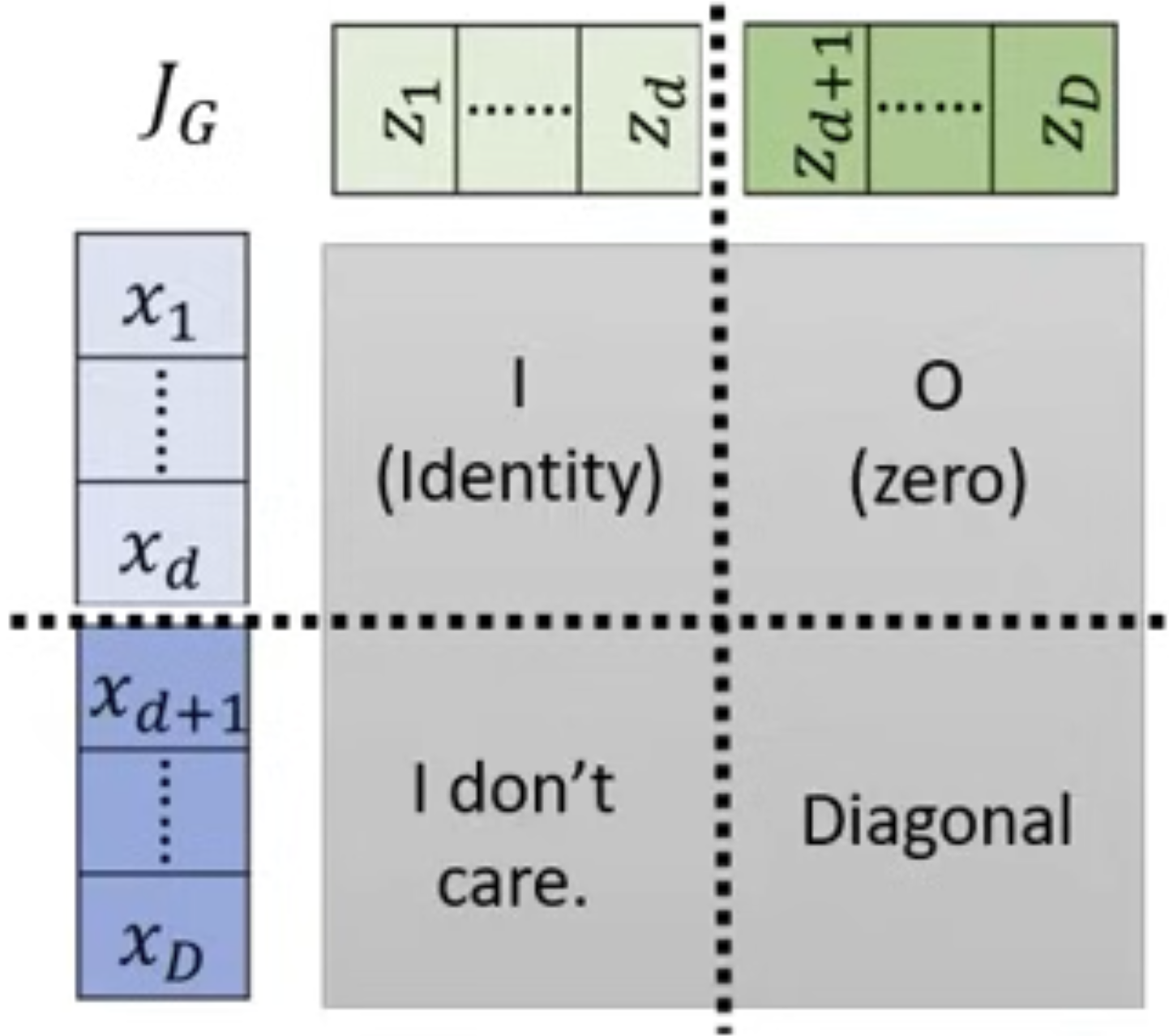
Determinant:

$$\det(J_G) = \prod_{i=d+1}^{D} \beta_i$$

Image:

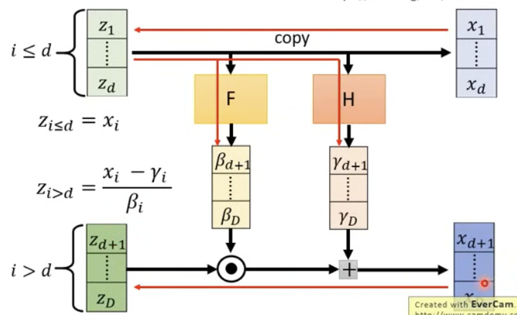
Determinant intuition:

Masking

Two masking strategies:

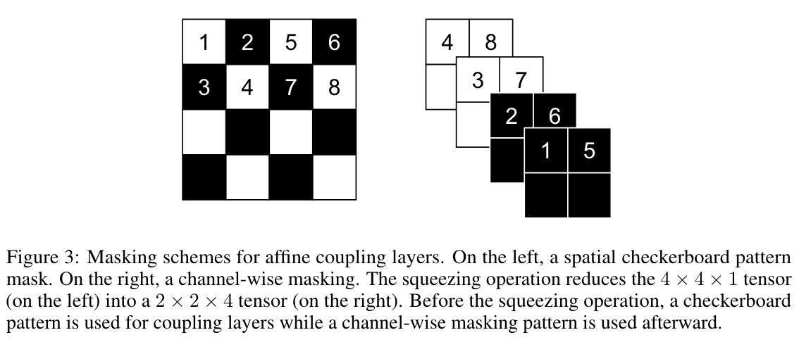
1. Checkerboard mask
2. Channel-wise masking (using squeezing to increase channels)

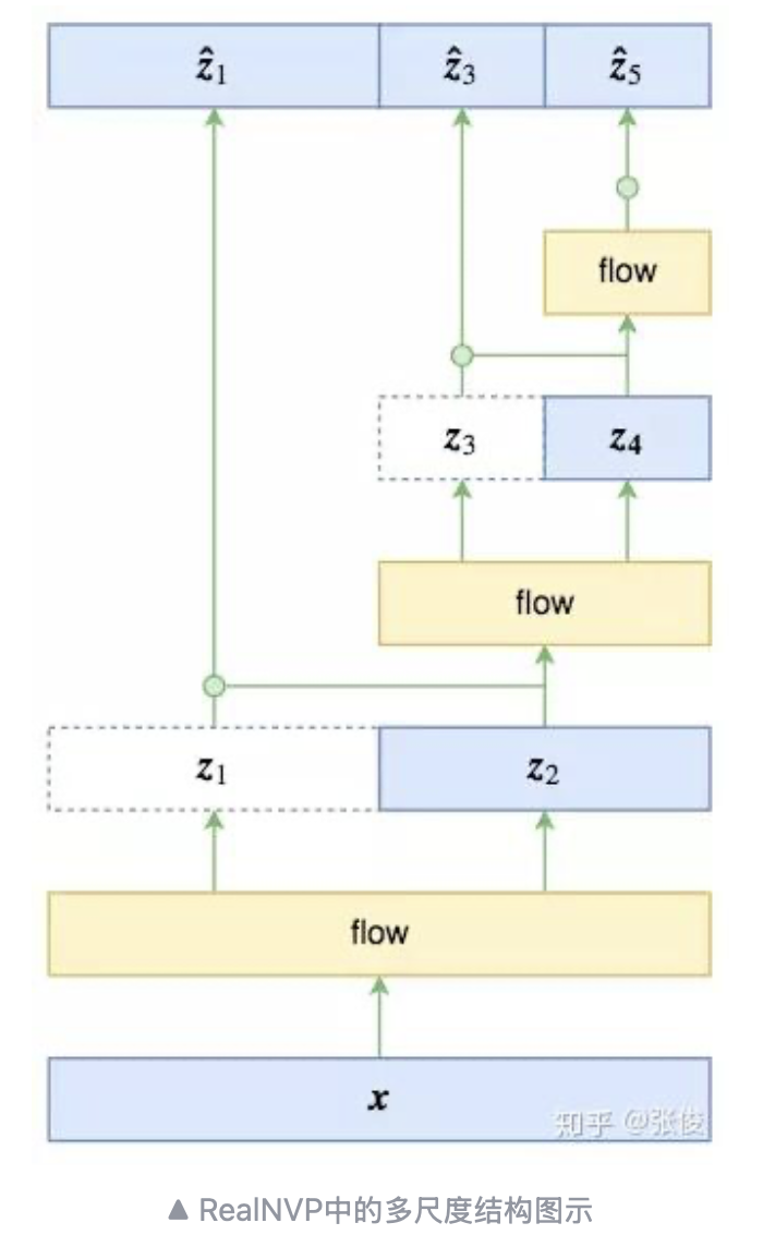
Composition of Coupling Layers

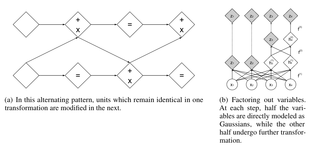
Multi-scale Architecture

Example structure:

• Variables at different scales are not equivalent
• Factorization:

$$p(z_1, z_3, z_5) = p(z_1|z_3,z_5)p(z_3|z_5)p(z_5)$$

Standardization:

$$\hat{z}_1 = \frac{z_1 - \mu(z_2)}{\sigma(z_2)}$$

Image:

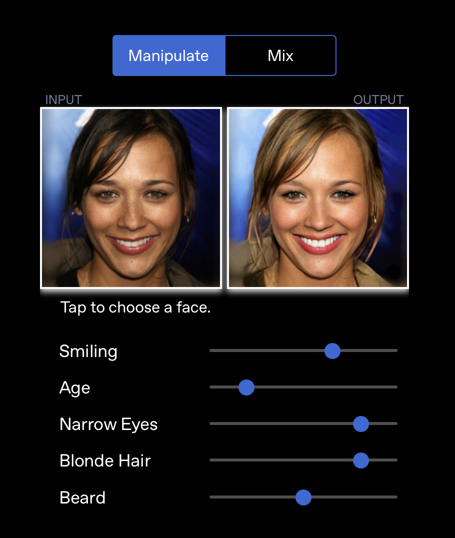
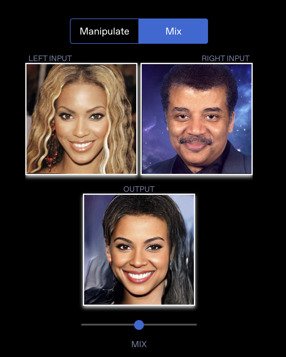
GLOW

Glow architecture:

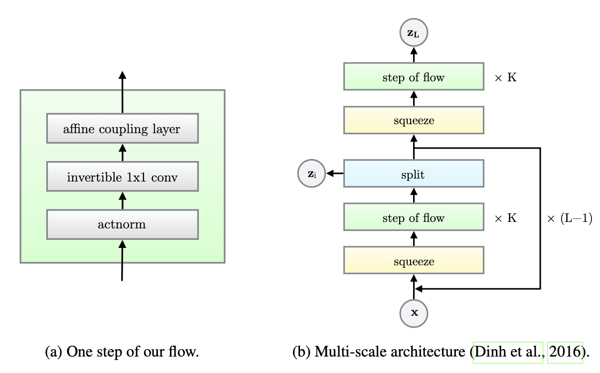
Glow properties:

Convolution as Invertible Transform

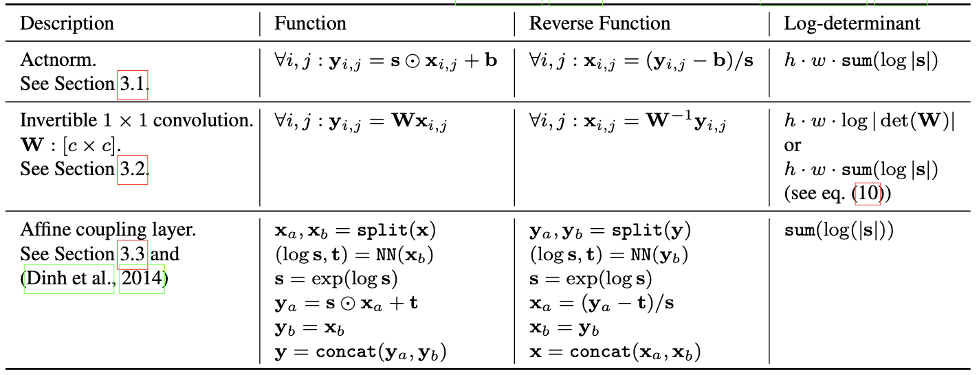
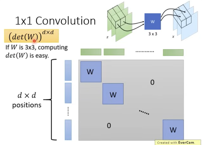
Channel mixing with invertible $3 \times 3$ matrix $W$:

$$x = Wz$$

If $W$ is invertible:

$$J_f = W$$

Image:

Results

See OpenAI Glow results: https://openai.com/index/glow/

---